Experiment 04: Classification Contract and Fixed Random Features

Experiment date: August 1, 2026
Distribution: Sensory 0.1.2 for Windows

Summary

Experiment 04 directly follows Experiment 03. It uses the same plant-watering decision problem, the same nine inputs, the same generator, the same balanced dataset, and the same safety policy in the PHP client.

It changes two essential elements:

1. instead of an almost identity-like hidden layer, it uses 128 fixed random nonlinear features;
2. instead of a generic text output, it uses a new explicit classification contract over real logits.

After 5,000 sample updates, model 04 reached 558/600, or 93.0%, on the included training dataset. The historically recorded result for Example 03 was 403/600, or 67.2%.

The experiment still does not use backpropagation through the hidden layer. Only the final classification readout and its biases are trained.

Experiment Question

Example 03 showed that merely inserting another layer does not guarantee better supervised learning. Its one-to-one transform only applied tanh to individual inputs and did not create new combinations of them. The final readout therefore remained effectively a shallow classifier.

Experiment 04 investigates:

• whether a fixed random-feature projection creates a more useful nonlinear representation;
• whether the LIGHT_WATER class becomes learnable with its own trainable bias;
• whether the trainer, saved network, and REST service use the same logits and probabilities;
• whether performance can be improved without claiming that Cognia supports end-to-end deep learning.

What Remains the Same as in Example 03

To keep the comparison understandable, the following elements were not changed:

• model and generator seed: 103;
• dataset: 600 examples, exactly 200 per class;
• nine input values;
• normalization of physical values to [-1, 1];
• one-hot representation of plant type;
• target classes NO_WATER, LIGHT_WATER, and DEEP_WATER;
• synthetic teacher and its decision thresholds;
• the direct raw skip path from inputs to the decision layer;
• deterministic safety rules in client.php;
• 5,000 sample-update steps for the main measurement.

The safety rules remain outside the neural network:

soil moisture >= 75%       -> NO_WATER
time since watering < 6 h  -> NO_WATER
highest confidence < 55%   -> WAIT_AND_RECHECK
otherwise                  -> network recommendation

The model therefore only recommends an action. A deterministic policy decides whether that action is permitted.

What Changed Compared with Example 03

1. Hidden Representation

Example 03 uses nine fixed one-to-one features:

9 inputs -> 9 independent tanh transforms -> 3 outputs

Each hidden neuron sees exactly one input. The layer therefore does not create combinations such as “dry soil together with high temperature and a low chance of rain.”

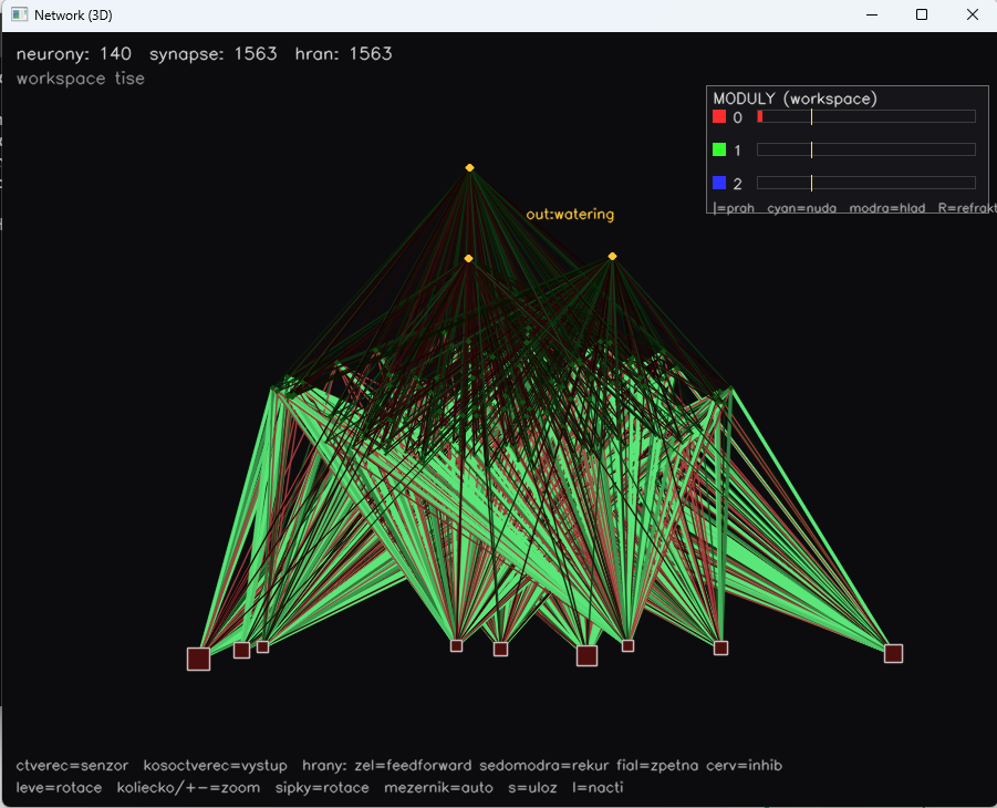
Example 04 uses 128 fixed random features:

                           +---------------- raw skip ----------------+
                           |                                          v
9 inputs -> 128 fixed random tanh features ----------------------> 3 logits

Each feature neuron is fully connected to all nine inputs with fixed random(-1.0, 1.0) weights. Its activation is a nonlinear projection of a combination of multiple inputs. This layer does not change during supervised training.

This follows the random-feature/ELM principle: a random nonlinear basis remains fixed, and only linear combinations over that basis are learned.

2. Topology Size

Property	Example 03	Example 04
Input neurons	9	9
Hidden neurons	9	128
Decision neurons	3	3
Total neurons	21	140
Synapses	63	1,563
Hidden projection	one-to-one	full random
Trained hidden layer	no	no

The higher performance of Example 04 therefore cannot be attributed only to the softmax correction. The model also has a substantially richer fixed representation.

3. Output Declaration

Example 03 declares a generic text output:

output text from brain.decision as watering {
    vocab: "no_water", "light_water", "deep_water";
}

text performs argmax over the normal dynamic neuron activations after tanh and leak. It is not a formal softmax classification head.

Example 04 declares a classification output:

output classification from brain.decision as watering {
    vocab: "no_water", "light_water", "deep_water";
    loss: softmax_cross_entropy;
}

This establishes an explicit contract:

• classification uses pre-tanh logits;
• the loss is softmax_cross_entropy;
• the trainer enables classification mode automatically;
• readout weights and one bias per class are trained;
• the trainer and REST service operate on the same logits.

4. Logit and Gradient Definition

The classification logit is:

logit_j = gain_j * acc_j / normalization(in_degree_j) + bias_j

Softmax is:

p_j = exp(logit_j) / sum_k(exp(logit_k))

The cross-entropy gradient with respect to a logit is:

dL/dlogit_j = p_j - target_j

The weight update accounts for the same gain and normalization as the forward pass:

delta_w = eta * pre * gain / normalization(in_degree) * (target - p)

The bias is trained separately:

delta_bias = eta * (target - p)

This is especially important for the middle LIGHT_WATER class. It must win between two decision boundaries; without independent intercepts, this type of interval problem is difficult to represent.

5. Authoritative Bias from Cognia

In the runtime used for Example 03, bias was present in the AST and topology but was not transferred into NeuralGraph; the GPU runtime created its own small random bias instead.

In the runtime used by Example 04, the declaration in the .cognia file is authoritative. The path is:

neuron state bias
    -> Topology
    -> MindSubstrate
    -> NeuralGraph::setNeuronBiases
    -> GPU dBias

After a checkpoint is loaded, its saved learned biases correctly override the initial values.

6. Independent Tabular Samples

Example 03 was trained inside the dynamic Mind without the tabular trainer always explicitly resetting activity between rows. Leak could carry some state from the previous sample.

In Example 04, cognia-dataset has a clear semantic contract: every row is an independent example. Activations and other dynamic state are reset before every sample, while learned parameters remain intact.

Sequential continuity remains available through the separate sequential mode and dataset format.

7. Deterministic Shuffling

Samples are deterministically shuffled after every pass. This reduces the effect of class ordering on the latest bias updates while keeping the result reproducible.

The value 5000 still means 5,000 sample-update steps, not 5,000 epochs. With 600 samples, this is approximately 8.33 passes through the dataset.

8. REST Contract and PHP Client

In Example 03, REST returns generic top-layer activations and the PHP client recomputes softmax over them. Those values need not be identical to those used by the supervised update.

Example 04 reads the named watering output from the outputs array. The server returns:

{
  "name": "watering",
  "type": "classification",
  "logits": [-4.2, 0.8, 5.1],
  "probabilities": [0.0001, 0.0133, 0.9866],
  "selected_index": 2,
  "selected_label": "deep_water",
  "confidence": 0.9866,
  "entropy": 0.071
}

The PHP client no longer recomputes softmax. It uses the probabilities and selected index returned directly by the server.

Example 04 Architecture

Input

The network receives nine values in this order:

1. soil moisture;
2. air temperature;
3. relative air humidity;
4. sunlight intensity;
5. rain probability;
6. hours since the last watering;
7. cactus indicator;
8. herb indicator;
9. tomato indicator.

The first six values are scaled to [-1, 1]; plant type is a one-hot vector.

Fixed Random-Feature Layer

The feature layer contains 128 neurons. Every neuron receives all nine inputs. The runtime divides accumulated input by the number of incoming edges, so a feature neuron uses gain: 9.0 to restore the scale of the sum.

The computation of one feature neuron is approximately:

feature_i = tanh(sum_j(w_ij * input_j) + bias_i)

Feature neurons have leak 0.10, but tabular state is reset before every sample and the forward pass is allowed to settle for several steps.

Classification Readout

Each of the three output neurons receives:

• 128 values from the random-feature layer;
• the nine original inputs through the raw skip path;
• its own trainable bias.

The total in-degree is 137, so the model uses gain: 137.0. This compensates for divisive normalization and makes the logit correspond to the sum of contributions rather than their mean.

Measurement Method

The main measurement uses:

.\cmake-build-debug\cognia_train.exe `
  .\Cognia\examples\04-classification-watering\watering.cognia `
  .\Cognia\examples\04-classification-watering\watering.dataset `
  5000 PlantWatering `
  --save .\Cognia\examples\04-classification-watering\watering.bin

The --softmax option is unnecessary: output classification enables softmax_cross_entropy automatically.

Measurements before and after training reset state for every sample and evaluate the classification head's actual logits.

Results

Example 04

Phase	Accuracy	Cross-entropy
Before training	151/600 = 25.2%	1.222745
After 5,000 updates	558/600 = 93.0%	0.170258

This means 407 additional correctly classified examples and an approximately 86% reduction in cross-entropy.

Comparison with Example 03

There are two useful reference points:

Variant	Runtime/training	Accuracy
Example 03, original historical measurement	original contract	403/600 = 67.2%
Example 03, control run on the corrected runtime	still output text, but corrected trainer	474/600 = 79.0%
Example 04	classification + 128 random features	558/600 = 93.0%

The Example 03 control run used the same 5,000 update steps and --softmax, while the Example 03 model file remained unchanged.

The table shows that:

• trainer and bias corrections alone raised the unchanged Example 03 model from approximately 67.2% to 79.0%;
• the explicit classification head and richer fixed representation in Example 04 added another 14 percentage points over the control run;
• the 03 -> 04 difference is not a clean ablation of one change, because both the output contract and fixed-feature capacity changed at the same time.

The MSE reported by Example 03 is not directly comparable with cross-entropy in Example 04. MSE was computed over dynamic activations, while Example 04 optimizes softmax cross-entropy over logits.

Deployment Verification

After saving and reloading watering.bin, the model was run through cognia_serve. Verified scenarios include:

Situation	Network / policy
dry tomato, hot weather, sunlight, almost no rain	DEEP_WATER, approximately 100%
cactus, medium moisture, likely rain	NO_WATER, approximately 99.9%
wet soil	NO_WATER, additionally confirmed by the safety override

This verifies the complete parse -> topology -> train -> save -> load -> REST -> PHP client path. The generated .bin is not a source artifact of the example.

What the Experiment Demonstrates

• declared bias is authoritative at runtime and classification biases are trained;
• the middle ordinal class is no longer structurally doomed to fail;
• the softmax-readout gradient matches the forward definition of a logit;
• independent tabular samples are not contaminated by state from the previous row;
• the trainer and REST service use the same logits and probabilities;
• fixed random features provide a practical supervised path without general autodiff;
• the safety policy can remain separate from the statistical model.

The separate Cognia/tests/12/classification.cognia regression test verifies a LOW/MID/HIGH problem, including the middle class. The project test suite requires it to reach at least 29/30.

What the Experiment Does Not Demonstrate

• This is not end-to-end training of the hidden layer.
• This is not general backpropagation through a Cognia DAG.
• This is not an agronomically validated model.
• The 93.0% result is training-dataset accuracy, not an estimate of generalization.
• Probabilities have not been calibrated on a separate validation set.
• Higher confidence does not automatically imply a safe decision.

Why the Result Is Not 100%

The synthetic teacher is deterministic, but its rules contain sharp combined conditions over demand score and rain probability. A finite fixed random basis only approximates them. Hidden weights do not adapt to classification error, and the readout uses a simple online gradient with bounded weights.

Diagnostic longer runs show that the model has not completely converged after 5,000 updates:

Update steps	Training accuracy	Cross-entropy
5,000	93.0%	0.170258
10,000	94.8%	0.150912
20,000	95.8%	0.115265

Chasing 100% on the same dataset is not the primary goal. It is more important to measure performance on a separate dataset generated with a different seed.

Meaningful Next Steps

1. Add a separate validation/test dataset with a different seed.
2. Report a confusion matrix and recall for every class.
3. Add --quiet, JSON metrics, and a clear distinction between update steps and epochs.
4. Compare 64, 128, and 256 random features on the same validation set.
5. Try a ridge/ELM readout solution or mini-batch optimization.
6. Calibrate confidence using validation data only.
7. Only then decide whether Cognia needs bounded backpropagation through an acyclic supervised DAG.

Conclusion

Example 04 addresses a concrete weakness exposed by Example 03 without pretending to perform deep learning. The fixed random-feature layer provides a richer nonlinear representation, and the explicit classification head unifies the mathematics of training and inference.

The 93.0% result is a substantial and reproducible improvement, but the correct interpretation is: Cognia now has a consistent and practically useful supervised classification head over a fixed representation. It does not mean that Cognia already supports general end-to-end supervised learning.