Polarized Neural Networks

Research concept

A polarized neural network is a proposed stateful neural architecture in which a neuron has not only an activation, bias, and synaptic weights, but also its own direction vector. A group of neurons simultaneously shares a dynamic polarization vector representing the current orientation of the entire computational region.

The central hypothesis is:

The same neural structure can perform a different computation over the same input depending on the direction of its continuously maintained polarization state.

The computation is therefore determined not only by input $x$ and weights $W$:

$$ y = F(x, W), $$

but also by the internal polarization state $\mathbf p_t$ and neuron orientations $D = {\mathbf d_i}$:

$$ (y_t, \mathbf p_{t+1}) = F(x_t, \mathbf p_t, W, D). $$

Polarization is neither another classification output nor a hidden switch. It is a continuous state that changes neuron sensitivity while simultaneously being changed by neuron activity. The network thereby becomes a dynamic system whose computation depends on the trajectory of its previous states.

Original motivation: mathematical use of the axon

The concept was originally inspired by the axon. In conventional computer neural networks, a neuron is reduced primarily to a scalar activation, and its axon has no geometric or directional meaning of its own. A biological axon carries a signal to other cells, but in an abstract model it usually disappears into a list of edges and weights.

A polarized network proposes using this omitted property mathematically. Each neuron $i$ receives a unit direction vector

$$ \mathbf d_i \in \mathbb R^2, \qquad |\mathbf d_i| = 1. $$

This vector can be understood as the neuron's abstract mathematical axon: it specifies neither the physical length nor the position of an axon, and it is not another synapse. It expresses the orientation in which the neuron agrees or disagrees with the state of the whole region.

The shared region vector

$$ \mathbf p_t \in \mathbb R^2 $$

occupies the same abstract directional space. It can be drawn in the plane of the polarized population in a visualization, but this geometry is primarily a representation of a mathematical relationship. The concept does not claim that biological axons implement the same two-dimensional polarization mechanism.

The contribution of the original axon intuition is the question of whether, in addition to connection strength, neuron orientation can serve as an independent computational parameter.

Polarization unit

A polarization unit is a group of neurons, typically a module or recurrent population. All neurons in the unit share one state $\mathbf p_t$, while each neuron has its own direction $\mathbf d_i$ and may have its own polarization strength $\alpha_i$.

The alignment of a neuron with the polarization is the dot product

$$ s_i = \mathbf d_i \cdot \hat{\mathbf p}_t, $$

where $\hat{\mathbf p}_t$ is the normalized polarization. For unit vectors, $s_i \in [-1,1]$:

$s_i \approx 1$: the neuron is aligned with the polarization;
$s_i \approx 0$: the neuron is neutral with respect to the polarization;
$s_i \approx -1$: the neuron is oriented against the polarization.

Polarization does not activate a neuron by itself. It modulates the effect of the actual synaptic input $z_i$:

$$ a_i = f!\left(z_i(1 + \alpha_i s_i) + b_i\right). $$

This distinction is important. Polarization does not carry content instead of synapses; it changes how the existing network processes content. The same input can therefore activate a different part of the population depending on prior context.

How polarization arises without a controller

In the autonomous variant, polarization emerges bottom-up from the activity of the population itself. Every active neuron contributes its direction. The current Cognia implementation uses activation magnitude so that positive and negative activations do not cancel each other:

$$ \mathbf c_t = \frac{\sum_i |a_i|\mathbf d_i} {\varepsilon + \sum_i |a_i|}. $$

The state then moves toward the resulting direction:

$$ \mathbf p_{t+1} = \operatorname{normalize}!\left( (1-\eta)\mathbf p_t + \eta\mathbf c_t \right), $$

where $\eta$ determines the rate of change. Optional momentum $\mu$ adds inertia:

$$ \mathbf v_{t+1} = \mu\mathbf v_t + \eta\mathbf c_t, $$

$$ \mathbf p_{t+1} = \operatorname{normalize}(\mathbf p_t + \mathbf v_{t+1}). $$

This creates a closed loop:

input and previous state
        ↓
neuron activations
        ↓
weighted sum of their “axon” directions
        ↓
new polarization of the region
        ↓
changed neuron sensitivity in the next step

Without a controller, polarization is an emergent state. The region interprets its own recent activity, and that interpretation influences its next response.

Appropriate uses without a controller

Autonomous polarization is suitable when state should arise directly from a sequence of observations:

retaining a latent interpretation of a sensor trajectory;
distinguishing situations with the same current input but different histories;
temporarily maintaining an expectation about the next sequence element;
stabilizing one of several dynamic regimes;
contextually modulating a recurrent reservoir;
representing a continuous automaton state without an explicit discrete switch.

Example 06 uses polarization to retain an interpretation of a lead vehicle's motion. After the informative part of the trajectory, both scenarios receive identical radar data. The polarized network nevertheless distinguishes for longer whether the vehicle had previously been slowing down or moving away. In a controlled ablation, it achieved 92.9% accuracy on the identical subsequent input, compared with 84.5% for the same network without polarization. This is an initial positive experimental signal, not yet a general proof of the architecture.

Risks of the autonomous variant

Polarization may collapse into nearly the same direction for every input.
It may merely duplicate ordinary recurrent memory without carrying independent information.
An excessively high $\eta$ causes instability, while an excessively low $\eta$ causes immobility.
Random directions $\mathbf d_i$ may fail to create a useful state space.
Strong modulation $\alpha$ may suppress input instead of processing it contextually.

Every experiment must therefore include an ablation with the same network and $\alpha=0$, and ideally variants with reset or randomly permuted $\mathbf p$.

Controller-driven polarization

In the second variant, a separate neural controller can propose the polarization direction. The controller observes selected context and emits two scalar outputs:

$$ \mathbf q_t = (q_x,q_y). $$

Normalization produces the requested direction $\hat{\mathbf q}_t$. It is blended with the autonomously computed polarization:

$$ \mathbf p_{t+1} = \operatorname{normalize}!\left( (1-k)\mathbf p_{t+1}^{\mathrm{intrinsic}}

k\hat{\mathbf q}_t \right), $$

where $k \in [0,1]$ is the control strength.

$k=0$: purely autonomous polarization;
$0<k<1$: the controller corrects the direction while the population retains its own dynamics;
$k=1$: the controller determines the resulting direction whenever its output is nonzero.

The Cognia interface is declared as follows:

controller PolarizationSteering {
    interface {
        observe observation[2];
        control polarization direction[2];
    }

    // Internal neural structure of the controller.
}

It is connected to a polarized module with:

control polarization of context.cells
    with steering.direction by 0.75;

The controller does not have to be an external algorithm. It is a neural network that can be learned from data. The result is a hierarchical architecture: one network does not directly determine another network's output, but instead sets its computational orientation.

What the controller adds

Without a controller, polarization answers:

Which regime naturally follows from the recent activity of this population?

With a controller, it answers:

In which regime should this population process its input now, given a broader context or objective?

The controller can thereby separate two timescales:

a fast network processes immediate sensor input;
a slower controller maintains the task, hypothesis, intention, or operating mode.

The same computational population can then be reused in several contexts without completely switching its weights.

Appropriate uses with a controller

Task conditioning: the same network solves different tasks according to the controller's objective.
Attention: the controller favors neurons oriented toward the relevant regime.
Working memory: a brief instruction establishes a direction that affects a long sequence of identical inputs.
Hierarchical control: a higher level selects the regime of a lower sensorimotor population.
Adaptive control: the controller switches between cautious, ordinary, and aggressive processing without directly generating the action output.
Hypothesis separation: the controller maintains an interpretation of the situation while the controlled population continues processing new data.

Example 07 uses a short MODE_X or MODE_Y instruction followed by inputs that are all identical. The controlled network retained 100% accuracy at the longest tested depths, 9–11, while the uncontrolled variant fell to 50%. Overall accuracy was nevertheless tied at 87.5%, because the controlled network made more transient errors at the beginning. The experiment therefore demonstrates longer mode retention but does not yet demonstrate higher average accuracy.

Risks of the controlled variant

The controller may solve the entire problem, making the polarized population redundant.
With $k=1$, the system may be only a complicated representation of a two-dimensional context input.
An incorrect controller may lock the whole population into an unsuitable regime.
If controller output and autonomous state are not measured separately, the source of an improvement cannot be identified.
Multiple controllers over one unit would create ambiguous competition; current Cognia therefore allows exactly one.

The controller's contribution must be tested against simpler alternatives: adding two ordinary input neurons, a gate mechanism, GRU/LSTM, a state-space model, and a larger recurrent reservoir.

Learning direction vectors

Directions $\mathbf d_i$ may be fixed random projections, but the concept's full potential lies in learning them. A local rule can attract an active neuron toward the direction of a successful state:

$$ \Delta \mathbf d_i = \eta_d r a_i \left( \hat{\mathbf p} - (\mathbf d_i\cdot\hat{\mathbf p})\mathbf d_i \right), $$

where $r$ is the reward, and subsequent normalization preserves $|\mathbf d_i|=1$. Positive reward stabilizes the orientation of neurons that contributed to a useful state; negative reward reorganizes it.

Another option is contrastive organization of the polarization space:

functionally similar contexts should have nearby polarizations;
different contexts should be separated by at least a chosen margin;
a correct stable polarization should not be penalized for changing little;
collapse of all sequences into one direction should be penalized.

From a scientific perspective, learning ordinary weights $W$, directional parameters $D$, the readout, and the controller must be separated. Otherwise it will be impossible to determine which part of the architecture produced the measured effect.

Difference from conventional mechanisms

Polarization shares goals with several established families of methods: recurrent state, gating, attention, neuromodulation, hypernetworks, and dynamic systems. The proposed mechanism seeks to distinguish itself through a specific parameterization:

each neuron has its own normalized orientation $\mathbf d_i$;
a population shares a low-dimensional directional state $\mathbf p$;
their dot product multiplicatively modulates neuron sensitivity;
population activity feeds back to create the next state $\mathbf p$;
an optional controller does not produce an action but controls the orientation of computation.

This parameterization alone does not establish scientific novelty. A systematic review of related models and peer-reviewed comparisons are required before claiming that this is a new type of neural network. This document therefore calls it a proposed concept, not a confirmed discovery.

What would constitute a genuine scientific contribution

The mere existence of another state vector is not sufficient. A scientific contribution would arise if experiments demonstrated at least one of the following properties:

Better memory efficiency: the same accuracy with fewer neurons or parameters than a comparable recurrent network.
Longer retention: slower information decay during identical or distracting subsequent input.
Faster mode adaptation: a small amount of data is sufficient for a controller to redirect an already learned population to a new task.
Compositional generalization: learned directions can be combined in previously unseen contexts.
Interpretability: trajectories of $\mathbf p_t$ consistently correspond to functional states and predict network behavior.
Local learning: directions can be learned effectively from local reward without full backpropagation through time.
Robust control: blending autonomous and controlled polarization outperforms both a purely autonomous network and a direct controller command.

The strongest result would not be a one-off accuracy increase, but a reproducible new tradeoff among capacity, memory duration, adaptability, and parameter count.

Minimal experimental methodology

Every experiment should use identical datasets, seed policy, parameter budget, and training budget. The minimum set of variants is:

Variant	Polarization	Controller	Purpose
A	disabled	no	ordinary recurrent baseline
B	autonomous	no	isolate the value of emergent state
C	controlled	yes	full proposed mechanism
D	disabled	direct context input	test whether adding two inputs is sufficient
E	random or permuted	no	test whether meaningful direction matters
F	autonomous, reset $\mathbf p$	no	prove that the network uses state history

Useful measurements include:

performance by temporal depth rather than only one average;
trajectories and separation of polarization states;
sensitivity to reset, rotation, and perturbation of $\mathbf p$;
parameter count and computation time;
results across multiple seeds with confidence intervals;
comparisons with GRU, LSTM, reservoir computing, and state-space models;
transfer to unseen lengths and combinations.

Falsifiable hypotheses

The concept has scientific value only if it can fail. The following hypotheses are directly testable.

H1 — Contextual causality

Given the same input $x_t$ and the same weights $W$, changing only $\mathbf p_t$ will produce a reproducibly different output.

H2 — Useful retention

After removal of informative input, a polarized network will retain information longer than a parameter-matched unpolarized network.

H3 — State-space structure

Functionally similar sequences will produce closer polarization trajectories than functionally different sequences, including on test data.

H4 — Benefit of control

A neural polarization controller will outperform directly adding the same two-dimensional signal to the controlled population's input.

H5 — Significance of neuron orientations

Randomly permuting or rotating learned $\mathbf d_i$ after training will degrade performance. If it does not, the “axon” directions are not functionally used.

If these hypotheses repeatedly fail, polarization is probably only a redundant representation of ordinary recurrent state.

Current state in Cognia

Cognia currently implements:

a two-dimensional direction $\mathbf d_i$ for each neuron;
shared state $\mathbf p$ for a module;
modulation strength alpha, update rate eta, and momentum mu;
autonomous polarization updates from absolute activation values;
local and contrastive learning of directions;
reset and observation of polarization state;
a neural control polarization port of width two;
blending of controller output with autonomous polarization;
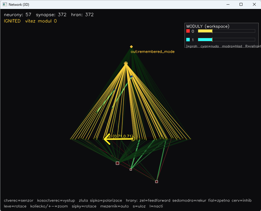
REST introspection and 3D visualization of the direction vector.

An autonomous unit is declared as follows:

module ContextArea {
    neurons { cells : Context[48]; }
    polarize {
        alpha: 0.9;
        eta: 0.5;
        mu: 0.0;
    }
}

The controller is optional. Without a control polarization ... command, the update remains fully autonomous.

Research interpretation

A polarized network can be understood as a low-dimensional state space embedded directly into a neuron population. The state is not merely a stored value beside the network. It has an immediate multiplicative relationship with every neuron through its “axon” direction, while neuron activity simultaneously rewrites it.

Without a controller, $\mathbf p$ is a memory of interpretation: the network creates its own orientation from history.

With a controller, $\mathbf p$ is a controlled computational regime: a higher neural structure determines how a lower structure should interpret subsequent input.

The original axon idea therefore does not mean simulating a biological axon literally. It means using the fact that a neuron can be mathematically enriched with an orientation that is absent from conventional computer models. If learned orientation proves to enable more efficient memory, control, or generalization, it may constitute an independent and scientifically testable contribution to neural architecture design.